Electoral College in Canada
This document simulates the US’ Electoral College, the system used to elect the President, in Canada. The data used is of the 2021 Federal Elections which re-elected Justin Trudeau to power. With the Electoral College, Trudeau would remain Prime Minister by a large margin.
The simulation was made originally for India (results here). Adapted on 26 June for Canada.
Process
The Electoral College is a system used in various countries to elect a President. This document focuses on the US implementation, which is the most widely-known. In this system, each state has a set number of votes, and all these votes go to the party which gets most votes.
- The Electoral College allots votes to each state somewhat proportional to their population
- Each Province gets a number of votes according to their population
- They also get an additional 2 votes, which comes from their representatives in the Senate
- In each state, the party with most votes gets all representatives in the College, regardless of their winning margin
Votes for a Province = Proportional Votes + 2 Senate VotesNote: Because all federal divisions in the US are states and have the same rights, they all have 2 seats in the Senate. In Canada, there are 3 Territories which have very small populations and have limited rights. To reflect this, they are not allotted any Senate seats.
Allotment
The seats allotted to each subdivision (10 Provinces + 3 Territories = 13 Federal Units):
stateInfo <- read.csv(params$STATES_PATH) %>% as_tibble()

addedSenateSeats <- params$SENATE_SEATS
perCapita <- sum(stateInfo$Population) / params$TARGET_VOTES

reps <- stateInfo %>%
  mutate(
    Number = ceiling(Population / perCapita) +
           case_when(Type == "Territory" ~ 0, TRUE ~ 2)
    ) %>%
  select(State, Population, Number)

kable(reps, col.names = c("Province", "Population", "Alotted Seats"))| Province | Population | Alotted Seats |
|---|---|---|
| ON | 14233942 | 41 |
| QC | 8501833 | 25 |
| NS | 969383 | 5 |
| NB | 775610 | 5 |
| MB | 1342153 | 6 |
| BC | 5000879 | 16 |
| PE | 154331 | 3 |
| SK | 1132505 | 6 |
| AB | 4262635 | 14 |
| NL | 510550 | 4 |
| NT | 41070 | 1 |
| YT | 40232 | 1 |
| NU | 36858 | 1 |
ps <- ggplot(reps) +
  geom_parliament(aes(seats = Number, fill = State)) +
  coord_fixed() +
  theme_void() +
  theme(legend.position = "bottom", plot.title = element_text(hjust = 0.5, face = "bold"), plot.subtitle = element_text(hjust = 0.5)) +
  guides(color = guide_legend(nrow = 2, byrow = TRUE)) +
  labs(
    legend = NULL,
    title = "Electoral College in Canada",
    caption = paste0("Total ", sum(reps$Number), " votes from ", length(stateInfo$State), " provinces and territories")
  ) +
  scale_fill_discrete(labels = reps$State)
ps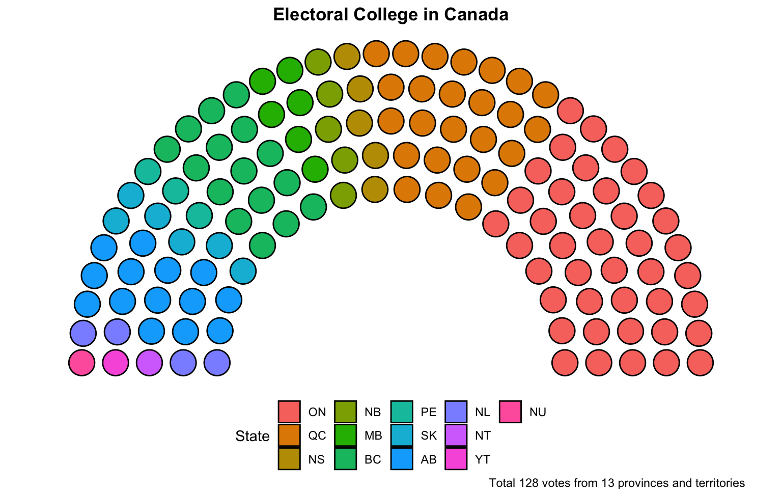
In the US, each vote ranges from representing almost 700,000 people in California to about 200,000 people in Wyoming.

options(scipen = 999)

plotData <- reps %>%
  arrange(desc(Population)) %>%
  mutate(PerCapita = Population / Number)
hPlot <- ggplot(plotData) +
  geom_bar(
    aes(x = reorder(State, -PerCapita), y = PerCapita),
    stat = "identity"
  ) +
  theme(axis.text.x = element_text(angle = 90, hjust = 1, size = 5)) +
  xlab("Province") +
  ylab("Voters per Rep")
ggplotly(hPlot)
In Canada, a vote in the Electoral College would go from representing 347,000 people in Ontario to 127,000 in Newfoundland and Labrador and just 51,000 in Prince Edward’s Island. PE and the territories together have 6 seats in the College, representing about 4.6% of total votes.
Results
This simulation assumes a broad alliance of left-wing and conservative parties, with the Liberals a senior partner in an alliance with the NDP and Greens, and the Conservatives the senior partner in an alliance with the People’s Party. The BCQ has not been included in any alliance.
preAllianceData <- data %>%
  group_by(Party, State) %>%
  summarise(TotalVotes = sum(Vote), .groups = "rowwise") %>%
  filter(!is.na(Party))
alliances <- read.csv(params$ALLIANCES_PATH) %>% as_tibble() %>% filter(Sc == 1)

alliancePreData <- tribble(~ Party, ~ State, ~ TotalVotes, ~ OriginalParty)
for (i in 1:length(preAllianceData$Party)) {
  pad <- preAllianceData[i,]
  ali <- which(alliances$Party == pad$Party)
  if (!identical(ali, integer(0))) {
    allianceEl <- alliances[ali,]
    alliancePreData <- alliancePreData %>%
      add_row(Party = allianceEl$Alliance, State = pad$State, TotalVotes = pad$TotalVotes, OriginalParty = pad$Party)
  } else {
    alliancePreData <- alliancePreData %>%
      add_row(Party = "Other", State = pad$State, TotalVotes = pad$TotalVotes, OriginalParty = pad$Party)
  }
}

stateWiseData <- alliancePreData %>%
  group_by(Party, State) %>%
  summarise(TotalVotes = sum(TotalVotes), .groups = "rowwise")

stateWinners <- tribble(~ Party, ~ State, ~ Votes)
for (state in unique(stateWiseData$State)) {
  stateData <- stateWiseData %>% filter(State == state)
  partyInfo <- stateData[which.max(stateData$TotalVotes),]
  stateWinners <- stateWinners %>% add_row(Party = partyInfo$Party, State = partyInfo$State, Votes = partyInfo$TotalVotes)
}


# Votes Calculation
preRes <- tribble(~ Party, ~ Votes)
for (state in unique(reps$State)) {
  iReps <- reps[which(reps$State == state),]
  iRes <- stateWinners[which(stateWinners$State == state),]
  preRes <- preRes %>% add_row(Party = iRes$Party, Votes = iReps$Number)
}

Results <- preRes %>%
  group_by(Party) %>%
  summarise(Votes = sum(Votes)) %>%
  mutate(Percent = sprintf((Votes / sum(Votes)) * 100, fmt = '%#.1f')) %>%
  arrange(desc(Votes)) %>%
  add_column(Colour = c("red", "blue"))
#add_column(Colour = c("orange", "green", "lightblue", "red", "cyan", "darkgreen", "pink", "black", "grey", "purple", "white"))

p <- ggplot(Results) +
  geom_parliament(aes(seats = Votes, fill = Party)) +
  coord_fixed() +
  theme_void() +
  theme(legend.position = "bottom", plot.title = element_text(hjust = 0.5, face = "bold"), plot.subtitle = element_text(hjust = 0.5)) +
  guides(color = guide_legend(nrow = 2, byrow = TRUE)) +
  labs(
    legend = NULL,
    title = "Electoral College in Canada",
    caption = paste0("Total ", sum(Results$Votes), " votes from ", length(stateInfo$State), " provinces and territories"),
    subtitle = paste0("", Results[1,]$Party, " wins with ", Results[1,]$Votes, " votes")
  ) +
  scale_fill_manual(values = Results$Colour, labels = Results$Party)
p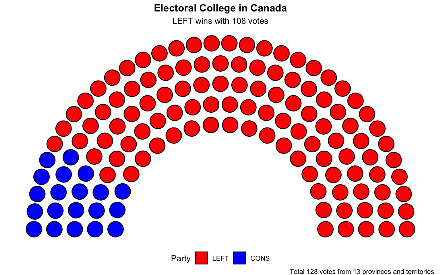
kable(Results %>% select(Party, Votes, Percent), col.names = c("Alliance", "Votes in the College", "Votes %"))| Alliance | Votes in the College | Votes % |
|---|---|---|
| LEFT | 108 | 84.4 |
| CONS | 20 | 15.6 |
The simulation results in the Left Alliance gaining every province and territory except Alberta and Saskatchewan, where the Conservative Alliance would win. Trudeau would receive 108 votes in the College, with Scheer managing to get just 20. Detailed results for each state below the map.
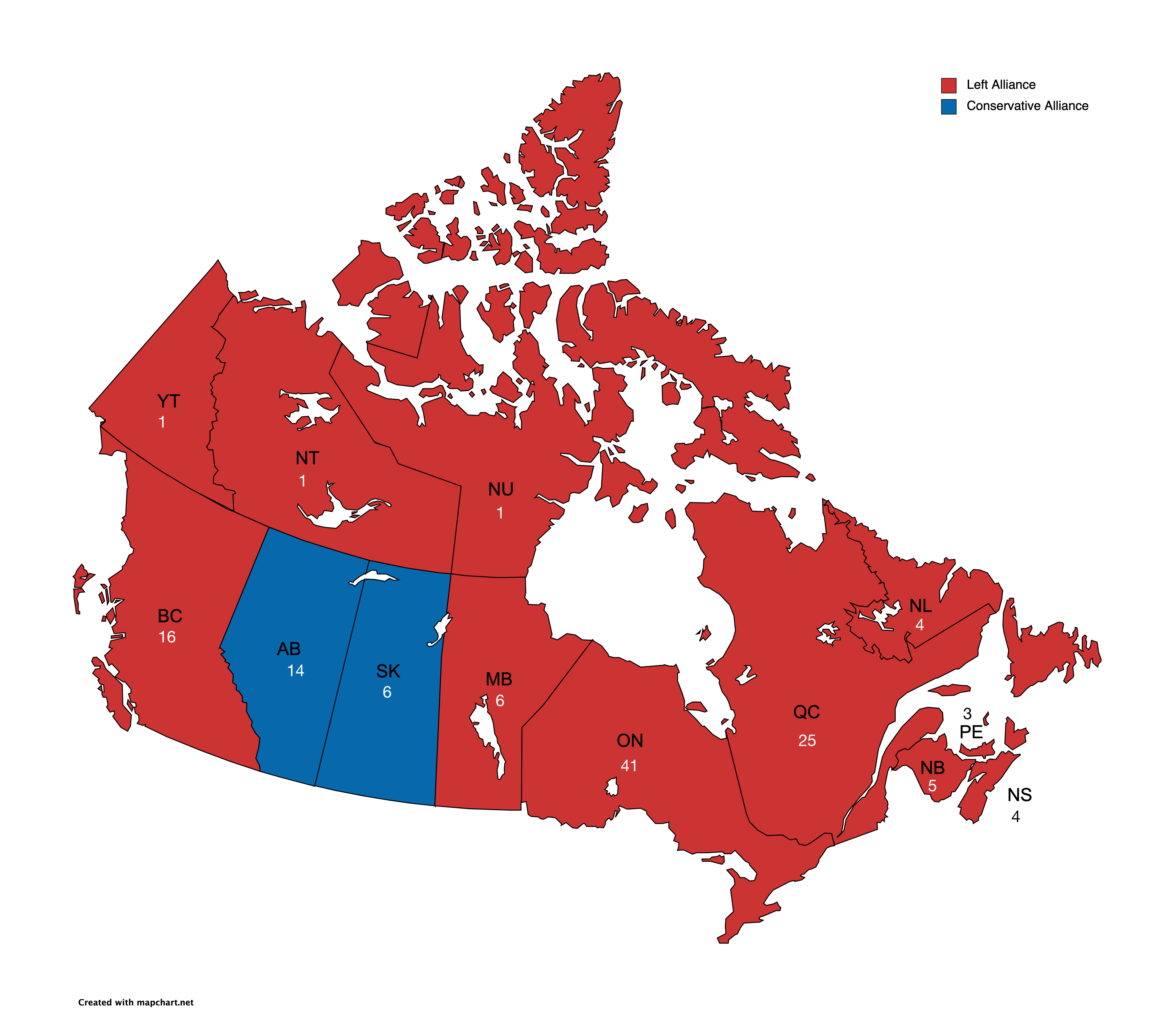
Provinces of Canada with Votes and Winners
detailed <- tribble(~ Province, ~ Winner, ~ WinnerVotes, ~ Opposition, ~ OppositionVotes)
for (state in unique(stateWiseData$State)) {
  sorted <- stateWiseData %>% filter(State == state) %>% arrange(desc(TotalVotes))
  winner <- sorted[1,]
  op <- sorted[2,]
  detailed <- detailed %>% add_row(Province = state, Winner = winner$Party, WinnerVotes = winner$TotalVotes, Opposition = op$Party, OppositionVotes = op$TotalVotes)
}

kable(detailed, col.names = c("Province", "Winner", "Vote %", "Runner Up", "Vote %"))| Province | Winner | Vote % | Runner Up | Vote % |
|---|---|---|---|---|
| AB | CONS | 62.7 | LEFT | 35.5 |
| BC | LEFT | 61.5 | CONS | 38.1 |
| MB | LEFT | 52.6 | CONS | 46.8 |
| NB | LEFT | 59.5 | CONS | 39.7 |
| NL | LEFT | 65.1 | CONS | 34.9 |
| NS | LEFT | 66.3 | CONS | 33.4 |
| NT | LEFT | 73.1 | CONS | 14.4 |
| NU | LEFT | 83.5 | CONS | 16.6 |
| ON | LEFT | 59.3 | CONS | 40.4 |
| PE | LEFT | 65.0 | CONS | 34.8 |
| QC | LEFT | 44.9 | BCQE | 32.1 |
| SK | CONS | 65.6 | LEFT | 32.8 |
| YT | LEFT | 60.3 | CONS | 26.2 |
Notes
Election data was sourced from Wikipedia, which sourced it from Elections Canada
Provinces/Territories and their population figures also obtained from Wikipedia, which sourced it from Statistics Canada
Graph and site generated with R and RMarkdown. Click on “Show all Code” at the top to view the source code for calculations.